AutoEncoder
AutoEncoder의 일반적인 의미는 "어떤 감독 없이도(즉, 레이블 되어 있지 않은 훈련 데이터를 사용해서) 입력 데이터의 효율적인 표현인 코드를 학습할 수 있는 인공 신경망"을 말한다. 구체적으로는 비지도 학습의 일환의 인공 신경망으로, 주어지는 Input 데이터에 대해 핵심적인 표현을 학습한 다음, 학습된 인코딩 표현에서 입력 데이터와 근사한 데이터를 Output으로 생성하는 것을 목표로 하는 생성 모델이다. 주로 주어진 데이터를 차원 축소를 통해 압축하여 차원의 저주 문제를 해결하거나 훈련 데이터의 증식을 위해 근사한 데이터를 생성 또는 중요한 feature를 찾아내는데에 활용된다. 이를 통해 해결할 수 있는 분야의 문제들은 여러가지가 있는데 대표적으로 Denoising, Outliar Detection 등이 있다. 여기서는 AutoEncoder의 여러 종류 중 Stacked AutoEncoder와 Denoising, Convolutional AutoEncoder를 다뤄보고자 한다.
Structure of AutoEncoder

일반적으로 AutoEncoder는 크게 인코더(Encoder)와 디코더(Decoder) 두가지 부분으로 구성되어 있다. 그림에서 볼 수 있듯이, 인코더와 디코더 사이에는 병목현상이 존재하는 은닉층이 들어간다. 이에따라 Encoder는 Input을 입력받아 이를 내부 표현으로 변환한다. 이 과정에서 데이터에 대한 주요 feature에 대해 학습이 진행되고, 해당 레이어를 거쳐 디코더를 통해 출력가능한 Output형태로 dimension을 펼치는 작용이 일어난다. 다시말해 인코더를 통해 압축된 데이터의 표현을 디코더가 해당 표현을 이용해 복원하는 역할을 한다고 볼 수 있다.
Stacked AutoEncoder
Stacked AutoEncoder는 여러개의 은닉층들을 가지며, 레이어를 추가할수록 AutoEncoder가 더 복잡한 표현을 학습할 수 있다. 다만, 레이어가 지나치게 많거나 노드수가 많아질 경우 AutoEncoder의 장점인 feature extraction이 올바르게 작용하지 못하고 지역적인 feature들을 추출하는 것과같은 과적합이 발생할 우려도 있어 적절한 hyper-parameter의 선정이 중요하다. Stacked AutoEncoder의 구조는 아래의 그림과 같이 가운데 은닉층을 기준으로 대칭인 구조를 가진다.

1. Simple AutoEncoder
1.1 Prepare
import numpy as np
import matplotlib
import matplotlib.pyplot as plt
import random
import os

import keras
from keras.datasets import mnist
from keras.models import Sequential
from keras.preprocessing import image
from keras.preprocessing.image import load_img,img_to_array
from keras.layers import Dense, Conv2D
# Load Data
train_set,test_set = mnist.load_data()
# Train - test split
X_train, Y_train = train_set
X_test, Y_test = test_set
print('Train, Test Data Shape:')
print(X_train.shape, Y_train.shape)
print(X_test.shape, Y_test.shape)# 행렬을 벡터화시킴
X_train_reshape=X_train.reshape((60000,28*28))
X_test_reshape=X_test.reshape((10000,28*28))
# Normalization
X_train_reshape=X_train_reshape/255
X_test_reshape=X_test_reshape/255
print('Train, Test Data Reshape:')
print(X_train_reshape.shape, Y_train.shape)
print(X_test_reshape.shape, Y_test.shape)Image 계열의 데이터 중 가장 기본이되는 mnist 데이터를 사용한다. keras를 통해 해당 데이터를 불러오고 적절한 shape으로 바꿔주는 reshape과정과 픽셀단위의 정규화를 실행해 일반적인 이미지 데이터 가공을 마쳤다.
1.2 Modeling to Fitting
# Create AutoEncoder Model
class AutoEncoder(keras.Model):
  def __init__(self, **setting):
    super(AutoEncoder, self).__init__(name=setting['model_name'])
    self.dense1 = Dense(units=setting['layer_size'], input_shape=(setting['input_shape'],),
                       activation=keras.activations.relu)
    self.dense2 = Dense(units=setting['output_shape'],
                       activation=keras.activations.sigmoid)

  def call(self, x):
    x = self.dense1(x)
    x = self.dense2(x)

    return x
2개의 Dense 레이어를 가지는 모델을 생성했다. 활성화 함수는 각각 relu와 sigmoid를 사용했다. 각종 hyper-parameter값은 setting이라는 변수로부터 입력받으며 Custom Model을 구현해 모델 사용의 재현성을 높였다.
setting = {
    'model_name': 'AE',
    'output_shape': 784,
    'input_shape': 784,
    'layer_size': 2
}

model = AutoEncoder(**setting)
model.compile(optimizer='adam',loss='mean_squared_error')

history = model.fit(X_train_reshape,X_train_reshape,epochs=20,validation_split=0.2)
. . .
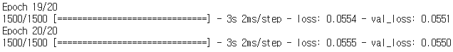
Fitting시 AutoEncoder의 정체성이 가장 크게 드러나는 부분이다. 일반적인 딥러닝 학습시 학습 대상인 입력변수 부분과 target label에 투입되는 데이터는 동일한 X_train 데이터이다. 즉, Input data를 보고 Input data로부터 학습하는 꼴이된다. 따라서 라벨링이 필요하지않은 온전한 비지도 학습방법이다. 이렇게 학습이 진행됨에따라 loss와 val_loss가 순차적으로 감소하는 것을 볼수 있으며 이는 네트워크가 Input data의 표현을 점차적으로 잘 이해해가고 있다는 것을 나타낸다.
1.3 Output Image & Extension
# Prediction
Output=model.predict(X_test_reshape)

# 인코더 결과를 출력 / Random한 5개 데이터 추출하여 사용
fig, axes = plt.subplots(2, 5, figsize=(10,5))

randomly_selected_imgs = random.sample(range(Output.shape[0]),5)
outputs = [X_test, Output]

# Original Input image & Output image
for row_num, row in enumerate(axes):
    for col_num, ax in enumerate(row):
        ax.imshow(outputs[row_num][randomly_selected_imgs[col_num]].reshape(28,28), cmap='gray')
        ax.grid(False)
        ax.set_xticks([])
        ax.set_yticks([])
plt.show()
해당 모델로 생성된 Output image는 위와 같다. 신경망의 층이 충분히 깊지 않아 제대로된 학습이 제대로 되지못해 아직 5와 8, 7과 9 등을 제대로 구분하지 못하는 등의 문제점들이 발견된 것을 볼 수 있다. 이에 따라 Dense층의 노드수를 증가시키며 출력되는 이미지를 비교했다.
# Plot the output from each model to compare the results
fig, axes = plt.subplots(6, 5, figsize=(15,15))

randomly_selected_imgs = random.sample(range(output_2_model.shape[0]),5)
outputs = [X_test, output_2_model, output_4_model, output_8_model, output_16_model, output_32_model]

# Iterate through each subplot and plot accordingly
for row_num, row in enumerate(axes):
    for col_num, ax in enumerate(row):
        ax.imshow(outputs[row_num][randomly_selected_imgs[col_num]].reshape(28,28), cmap='gray')
        ax.grid(False)
        ax.set_xticks([])
        ax.set_yticks([])

plt.show()
첫번째 Dense층의 노드수를 2부터 32까지 2의 제곱수로 변화시키며 출력되는 이미지를 순차적으로 출력했다. Mnist 데이터는 흑백으로 이루어진 필기체 형식의 비교적 간단한 이미지이므로 추가적인 적층없이 노드 수의 조절만으로도 어느정도 유사성이 높은 이미지를 생성해낼 수 있다. 원본 이미지와 비교해보았을때 노드수가 많아질 수록 점차적으로 5와 9에 대한 구분, 6과 8에 대한 구분이 명확해진다.
2. Denoising AutoEncoder
# Instill random noise
X_train_noised=X_train_reshape+np.random.normal(0,0.5,size=X_train_reshape.shape)
X_test_noised=X_test_reshape+np.random.normal(0,0.5,size=X_test_reshape.shape)

# Normalization
X_train_noised=np.clip(X_train_noised,a_min=0,a_max=1)
X_test_noised=np.clip(X_test_noised,a_min=0,a_max=1)

# Noise data
plt.imshow(X_train_noised.reshape(60000,28,28)[0],cmap='gray')
동일한 mnist 데이터에 random noise를 추가했다. 마찬가지로 정규화 과정을 거치고 이를 target데이터로 사용해 원본 데이터를 Input으로 입력받아 해당 noise를 제거하는 Denoising의 과정을 수행한다. 모델은 위에서 사용한 모델과 동일한 32개의 노드를 가진 2개의 레이어로 구성된 모델을 사용했다.
# Prediction
Output=model.predict(X_test_noised)

# Visualization
fig, ((ax1, ax2, ax3, ax4, ax5), (ax6, ax7, ax8, ax9, ax10), (ax11,ax12,ax13,ax14,ax15)) = plt.subplots(3, 5, figsize=(10,5))
randomly_selected_imgs = random.sample(range(Output.shape[0]),5)

# Original image
for i, ax in enumerate([ax1,ax2,ax3,ax4,ax5]):
    ax.imshow(X_test_reshape[randomly_selected_imgs[i]].reshape(28,28), cmap='gray')
    if i == 0:
        ax.set_ylabel("Original \n Images")
    ax.grid(False)
    ax.set_xticks([])
    ax.set_yticks([])

# Noise image
for i, ax in enumerate([ax6,ax7,ax8,ax9,ax10]):
    ax.imshow(X_test_noised[randomly_selected_imgs[i]].reshape(28,28), cmap='gray')
    if i == 0:
        ax.set_ylabel("Input With \n Noise Added")
    ax.grid(False)
    ax.set_xticks([])
    ax.set_yticks([])

# Denoising output image
for i, ax in enumerate([ax11,ax12,ax13,ax14,ax15]):
    ax.imshow(Output[randomly_selected_imgs[i]].reshape(28,28), cmap='gray')
    if i == 0:
        ax.set_ylabel("Denoised \n Output")
    ax.grid(False)
    ax.set_xticks([])
    ax.set_yticks([])

plt.show()
노이즈가 추가된 이미지를 훈련된 모델에 입력하면 위와 같이 노이즈가 제거된 이미지를 얻을 수 있다. 마찬가지로 네트워크가 충분히 깊지않아 완벽한 노이즈의 제거는 되지않았으나 레이어 수를 늘려 깊은 네트워크를 만들면 더 완벽한 Denoising Image를 얻을 수 있다. 현재 예시에서는 임의로 random noise를 추가해 target 데이터로 이용했지만 다음에서는 인위적인 noise가 아닌 실제 데이터를 사용하고 모델의 깊이와 유형을 변화시켜 유의미한 성능의 개선을 보여주고자한다.
3. Convolutional Stacked AutoEncoder
이번에는 Convolutional Layer를 사용해 인코더 및 디코더 레이어를 여러 층으로 적재한 AutoEncoder를 통해서 Denoising을 해보고자한다. 기존 Dense Layer를 사용한 것과 다르게 이미지 문제에서 좋은 결과를 보여주는 것으로 알려진 Convolutional Layer를 이용하며 더 깊은 네트워크 구조를 가진다. 사용하는 이미지 데이터는 다음과 같다.


# Modeling
conv_autoencoder=Sequential()

# Encoding
conv_autoencoder.add(Conv2D(filters=32,kernel_size=(3,3),input_shape=(420,540,1),activation='relu',padding='same'))
conv_autoencoder.add(Conv2D(filters=16,kernel_size=(3,3),activation='relu',padding='same'))
conv_autoencoder.add(Conv2D(filters=8,kernel_size=(3,3),activation='relu',padding='same'))

# Decoding(들어온 그대로 거꾸로 펼침)
conv_autoencoder.add(Conv2D(filters=8,kernel_size=(3,3),activation='relu',padding='same'))
conv_autoencoder.add(Conv2D(filters=16,kernel_size=(3,3),activation='relu',padding='same'))
conv_autoencoder.add(Conv2D(filters=32,kernel_size=(3,3),activation='relu',padding='same'))

# 출력층
conv_autoencoder.add(Conv2D(filters=1,kernel_size=(3,3),activation='sigmoid',padding='same'))

conv_autoencoder.summary()
인코더와 디코더 모두 각각 3개의 층을 가진다. 모든 층의 kernel size는 3x3이며 filter는 32, 16, 8, 8, 16, 32로 둘의 구조는 완벽하게 대칭구조를 가지고있어 인코더에서 입력받은 그대로 디코더를 통해 차원을 펼쳐주며 마지막에는 출력층을 통해 이미지를 생성한다.
conv_autoencoder.compile(optimizer='adam',loss='binary_crossentropy')
conv_autoencoder.fit(X_train_noisy,X_train_clean,epochs=10)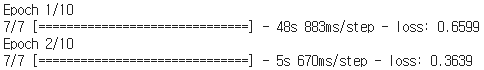
. . .

Mnist의 경우와는 다르게 여기서 loss function은 mse가 아닌 binary crossentropy를 사용했다. Cross Entropy는 일반적으로 2개의 값 사이에서 차이를 구한다. Mean Square Error의 경우는 다수의 정보로부터 적절한 근사값을 구한 것이 목적이다. Cross Entropy 는 각각의 표현되는 특징이 똑같은 지를 검증하는 함수이며, Mean Square Error는 특징들이 구성된 하나의 데이터, Object 등을 비교할 때 쓰는 함수이다. 두가지 loss function 모두 생성적인 모델에서 대표적으로 사용되는 함수들이다.
# Prediction
output=conv_autoencoder.predict(X_test_noisy)

# Plot Output
fig, ((ax1,ax2,ax3),(ax4,ax5,ax6)) = plt.subplots(2,3, figsize=(10,5))

randomly_selected_imgs = random.sample(range(X_test_noisy.shape[0]),2)

for i, ax in enumerate([ax1, ax4]):
    idx = randomly_selected_imgs[i]
    ax.imshow(X_test_noisy[idx].reshape(420,540), cmap='gray')
    if i == 0:
        ax.set_title("Noisy Images")
    ax.grid(False)
    ax.set_xticks([])
    ax.set_yticks([])

for i, ax in enumerate([ax2, ax5]):
    idx = randomly_selected_imgs[i]
    ax.imshow(X_test_clean[idx].reshape(420,540), cmap='gray')
    if i == 0:
        ax.set_title("Clean Images")
    ax.grid(False)
    ax.set_xticks([])
    ax.set_yticks([])

for i, ax in enumerate([ax3, ax6]):
    idx = randomly_selected_imgs[i]
    ax.imshow(output[idx].reshape(420,540), cmap='gray')
    if i == 0:
        ax.set_title("Output Denoised Images")
    ax.grid(False)
    ax.set_xticks([])
    ax.set_yticks([])

plt.tight_layout()
plt.show()
Output Denoised Image를 보면 Clean Images와 비교했을때 모든 글자들이 완벽하게 복원되고 있음이 보인다. Mnist 데이터와 다르게 Denoising의 정확성과 강도가 높아졌다. 이렇게 Convolutional Layer를 이용하면 일정한 분포에서 추출한 random noise가 아닌 구겨지거나 물들은 듯한 불특정한 noise에서도 깔끔한 이미지를 추출해낼 수 있다. 또한 위와 같이 학습된 모델을 Feature Extractor로 활용해 다른 도메인의 Denoising 문제에도 쉽게 적용할 수있는 장점이 있다.
'Deep Learning > Vision' 카테고리의 다른 글
| Image Classification < Basic To Transfer > - (3) (0) | 2021.04.05 |
|---|---|
| Image Classification < Basic To Transfer > - (2) (0) | 2021.04.01 |
| Image Classification < Basic To Transfer > - (1) (0) | 2021.03.27 |


